The purpose of this tutorial is to understand PCA and to be able to carry out the basic visualizations associated with PCA in R.
What is the purpose of PCA?
In two words: dimensionality reduction. Basically, PCA uses linear algebra to transform the original variables into a new set of variables called Principal Components (PCs). The number of original observations and variables stays the same, but the new variables are ordered by how much variance they explain in the data. This data matrix D is an N x P matrix, with each row corresponding to one of N samples/observations, and each of P variables as columns.
- The covariance between two normalized variables is the correlation coefficient.
How do we conduct PCA in R?
- First, we need some data,
d.
d = matrix(rnorm(40, 4, 5), nrow = 10, ncol = 4)
rownames(d) = paste0("Pt_", letters[1:10])
colnames(d) = paste0("Var_", 1:4)
d #a matrix with 10 observations and 4 variables
## Var_1 Var_2 Var_3 Var_4
## Pt_a -1.9558275 8.222110 6.1330495 -1.2082569
## Pt_b 0.1550978 8.926177 12.3491093 2.8760509
## Pt_c 7.9871980 3.500382 0.6552243 8.8333757
## Pt_d 3.4647598 5.172815 7.9080470 6.7127816
## Pt_e 0.7800012 9.318161 7.4073449 1.2008002
## Pt_f 3.7687596 1.723963 13.7647090 -2.2736195
## Pt_g -0.2716838 9.918819 15.5348005 1.4704897
## Pt_h -5.6275395 4.241205 3.8511981 8.5292215
## Pt_i 7.1371346 3.880500 2.3183988 -0.4720483
## Pt_j -7.9964361 -1.353237 4.6886856 5.8758227In this case, we have 10 patients (observations), Pt_1 through Pt_10, and 4 variables, Var_1 through Var_4. These variables are gene expression levels from 4 genes measured from each patient’s blood.
- Our next step is to standardize our variables. This includes, for each variable, centering the mean around 0 and scaling the variance to equal 1. Depending on your data, a log, Box-Cox, or other transformation may be required to make the variables look more like a standard normal distribution. Why? PCA works best when the variables have a joint multivariate Normal (Gaussian) distribution, though this does not stop you from applying PCA to non-normal data, such as genotype data (which consists of the integers 0, 1, & 2).
dctr = apply(d, 2, function(x) x - mean(x)) #mean-center the variables
dctr.std = apply(dctr, 2, function(x) x / sd(x))- Next, we calculate the covariance of
dctr.std, and observe that it is equivalent to the correlation matrix when the variables have a mean of 0 and standard deviation 1. Note that the variance of each variable is shown along the main diagonal, and the covariance of each variable with the other variables is shown in the off diagonal.
dctr.std.c = cov(dctr.std)
dctr.std.c #same as cor matrix with unit std dev & 0 mean
## Var_1 Var_2 Var_3 Var_4
## Var_1 1.00000000 0.1003648 -0.09638971 -0.1770692
## Var_2 0.10036483 1.0000000 0.42300878 -0.2901988
## Var_3 -0.09638971 0.4230088 1.00000000 -0.4839073
## Var_4 -0.17706923 -0.2901988 -0.48390733 1.0000000all.equal(dctr.std.c, cor(dctr.std))## [1] TRUEThere are two important things to note about the dctr.std.c covariance matrix:
- 1. It is square (\(P x P\)). This means that we can apply techniques that describe square matrices, such as eigenvalues and eigenvectors (Step 4). Note that the eigenvalues are closely related to the trace, determinant, and rank, all of which are additional features of square matrices.
- 2. It is symmetric (dctr.std.c = t(dctr.std.c)) about the diagonal. It is also positive semi-definite, which is a common type of matrix in statistics to compute on.
- The next step is to extract the eigenvalues & eigenvectors of the covariance matrix
dctr.std.c. We do that in 1 step witheigen.
d.c.e = eigen(dctr.std.c)

pca = prcomp(dctr.std)- We’ll then inspect the eigenvectors. There should be as many eigenvectors as there are original variables, and the eigenvectors are all perpendicular to each other. The length of the eigenvector is 1, by convention. This is similar to pythagoras’ theorem, whereby the sum of the squares gives you the Euclidian distance (L2 norm)
## first we look at the eigenvectors of the covariance matrix.
## each column in this matrix is an eigenvector
d.c.e$vectors
## [,1] [,2] [,3] [,4]
## [1,] -0.1194982 0.935008715 0.04860983 0.3303271
## [2,] -0.5348205 -0.001424129 0.78784976 -0.3053814
## [3,] -0.6060589 -0.322789854 -0.13512076 0.7143120
## [4,] 0.5765239 -0.146844765 0.59889249 0.5360826sqrt(sum(d.c.e$vectors[,1]^2)) #length of 1st eigenvector = 1## [1] 1sqrt(sum(d.c.e$vectors[,2]^2)) #length of 2nd eigenvector = 1## [1] 1## the dot product of any 2 eigenvectors is 0
## which means they are perpendicular to each other
d.c.e$vectors[,1] %*% d.c.e$vectors[,2]## [,1]
## [1,] -1.94289e-16- Another name for the covariance matrix
dctr.std.cis the transformation matrix, which transforms the coordinate space. We are looking for column vectors (eigenvectors) ofd.c.ethat, when multiplied on the right of the covariance (transformation) matrix, yield the same vector, but scaled. The degree to which they are scaled are the eigenvalues. This is the same as saying \(A\lambda = c\lambda\), where c is a constant equal to the eigenvalue. A is the transformation matrix, and lambda is the eigenvector. This is illustrated below with the first eigenvector/value:
## the covariance of the data * the 1st eigenvector...
dctr.std.c %*% matrix(d.c.e$vectors[,1], ncol=1)
## [,1]
## Var_1 -0.2168421
## Var_2 -0.9704887
## Var_3 -1.0997584
## Var_4 1.0461640##...equals the scale factor * the 1st eigenvector
d.c.e$values[1] * matrix(d.c.e$vectors[,1], ncol=1) ## [,1]
## [1,] -0.2168421
## [2,] -0.9704887
## [3,] -1.0997584
## [4,] 1.0461640- We’ll now inspect the eigenvalues of the covariance matrix. The eigenvalues are linearly decreasing, positive numbers. The normalized sum of the eigenvalues represents the variance explained by each eigenvector.
#eigenvalues
d.c.e$values
## [1] 1.8146064 1.0609325 0.7130462 0.4114149#plot the percent variance explained by each PC
perc_var <- d.c.e$values/sum(d.c.e$values)
plot(1:length(perc_var), perc_var, xlab="index", ylab="% variance")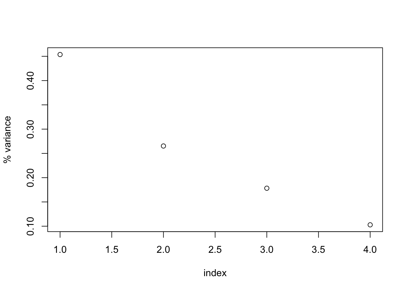
- Now that we have these eigenvectors (ie new orthogonal coordinates that describe the variance in the data), we must transform our original data into this new coordinate space. Our new data will have the same dimensions. To do this, we’ll multiply our the original scaled dataset by the eigenvectors. If we wanted only 2 variables (for visualization purposes) we could also do that.
## centered variables * eigenvectors
## should equal prcomp(dctr.std)$x
new.vars = dctr.std %*% d.c.e$vectors

## This works too:
## new.vars.3 = dctr.std %*% d.c.e$vectors[1:3,]- There are a few interesting properties of these new variables. First, these new variables are all uncorrelated with each other, as can be seen with the 0’s in the off diagonals in the covariance matrix. The variance of each new variable can be found in the diagonal entries in the covariance matrix between all values. The variance of each variable is also equal to the eigenvalues. Each variable is still centered at 0 as well.
#all the new variables are uncorrelated (0 covariance!)
round(cov(new.vars), 3)
## [,1] [,2] [,3] [,4]
## [1,] 1.815 0.000 0.000 0.000
## [2,] 0.000 1.061 0.000 0.000
## [3,] 0.000 0.000 0.713 0.000
## [4,] 0.000 0.000 0.000 0.411var(new.vars[,1])## [1] 1.814606d.c.e$values## [1] 1.8146064 1.0609325 0.7130462 0.4114149cov(prcomp(dctr.std)$x) #this is the same as the line above## PC1 PC2 PC3 PC4
## PC1 1.814606e+00 2.332962e-16 -7.530386e-17 1.269924e-16
## PC2 2.332962e-16 1.060932e+00 -1.049267e-17 2.589090e-16
## PC3 -7.530386e-17 -1.049267e-17 7.130462e-01 5.532217e-17
## PC4 1.269924e-16 2.589090e-16 5.532217e-17 4.114149e-01diag(prcomp(dctr.std)$sdev^2) #this is the same as the line above## [,1] [,2] [,3] [,4]
## [1,] 1.814606 0.000000 0.0000000 0.0000000
## [2,] 0.000000 1.060932 0.0000000 0.0000000
## [3,] 0.000000 0.000000 0.7130462 0.0000000
## [4,] 0.000000 0.000000 0.0000000 0.4114149colSums(new.vars) #equal 0, so these are still 0-centered!## [1] 1.443290e-15 1.249001e-16 -7.771561e-16 3.885781e-16- So we performed a linear transformation of our original scaled variables into this new coordinate space. Shouldn’t we be able to transform these variables back into the original scaled variables? Yes!
## how do we get back the original data from eigenvectors/values?
## multiply the eigenvectors by the rotated variables
all.equal(t(d.c.e$vectors %*% t(new.vars)), dctr.std)
## [1] "Attributes: < Component \"dimnames\": Component 2: target is NULL, current is character >"## returns the original data
all.equal(t(d.c.e$vectors %*% t(new.vars))+ d - dctr.std, d)## [1] "Attributes: < Component \"dimnames\": Component 2: target is NULL, current is character >"- Here are a few things to remember about linear transformations:
- Linear transformations are the specialty of linear algebra (as opposed to nonlinear transformations)
- Linear transformations are represented by matrices, known as transformation matrix (TMs).
- TMs, when multiplied to the left of vectors that have unit variance, transform the vector into the new transformed coordinate space (e.g. shear in 2d)
- The covariance matrix functions as a transformation matrix.
- The whole pca procedure can be implemented with built in functions in R or by using the singular value decomposition on the covariance matrix.
pca = prcomp(d, center = T, scale. = T)
all.equal(pca$rotation %*% t(pca$x) , t(dctr.std))
## [1] TRUE#these are almost equal, the 1st column of pca$x is *-1
#of the 1st column of new.vars
pca$x; new.vars## PC1 PC2 PC3 PC4
## Pt_a 0.8081307 0.25155503 -0.01855262 1.17528184
## Pt_b 1.1365823 0.41508833 0.58354034 -0.32932297
## Pt_c -1.7289742 -1.56004385 0.69134806 -0.39400744
## Pt_d -0.4117956 -0.34023509 0.49756293 -0.72261493
## Pt_e 0.8449073 -0.07886667 0.56082667 0.59019993
## Pt_f 1.0773813 -0.34209762 -1.71445030 -0.68402661
## Pt_g 1.8560070 0.64884427 0.49868111 -0.49066513
## Pt_h -1.5085981 1.12427012 0.58894235 0.12904804
## Pt_i -0.1758925 -1.63216243 -0.64758401 0.67795724
## Pt_j -1.8977483 1.51364790 -1.04031453 0.04815002## [,1] [,2] [,3] [,4]
## Pt_a -0.8081307 -0.25155503 -0.01855262 -1.17528184
## Pt_b -1.1365823 -0.41508833 0.58354034 0.32932297
## Pt_c 1.7289742 1.56004385 0.69134806 0.39400744
## Pt_d 0.4117956 0.34023509 0.49756293 0.72261493
## Pt_e -0.8449073 0.07886667 0.56082667 -0.59019993
## Pt_f -1.0773813 0.34209762 -1.71445030 0.68402661
## Pt_g -1.8560070 -0.64884427 0.49868111 0.49066513
## Pt_h 1.5085981 -1.12427012 0.58894235 -0.12904804
## Pt_i 0.1758925 1.63216243 -0.64758401 -0.67795724
## Pt_j 1.8977483 -1.51364790 -1.04031453 -0.04815002#svd on covariance matrix
dctr.c.svd = svd(dctr.std.c)
all.equal(dctr.c.svd$d, d.c.e$values) #eigenvalues, same as d.c.e$values## [1] TRUE#these are almost equal, one is the negative of the other
dctr.c.svd$u; d.c.e$vectors## [,1] [,2] [,3] [,4]
## [1,] -0.1194982 0.935008715 -0.04860983 -0.3303271
## [2,] -0.5348205 -0.001424129 -0.78784976 0.3053814
## [3,] -0.6060589 -0.322789854 0.13512076 -0.7143120
## [4,] 0.5765239 -0.146844765 -0.59889249 -0.5360826## [,1] [,2] [,3] [,4]
## [1,] -0.1194982 0.935008715 0.04860983 0.3303271
## [2,] -0.5348205 -0.001424129 0.78784976 -0.3053814
## [3,] -0.6060589 -0.322789854 -0.13512076 0.7143120
## [4,] 0.5765239 -0.146844765 0.59889249 0.5360826- Scatterplot of new variables
plot(new.vars[1,], new.vars[2,], xlab=paste0("PC1: ", round(perc_var[1],2)*100, "% of variance"), ylab=paste0("PC2: ", round(perc_var[2],2)*100, "% of variance"))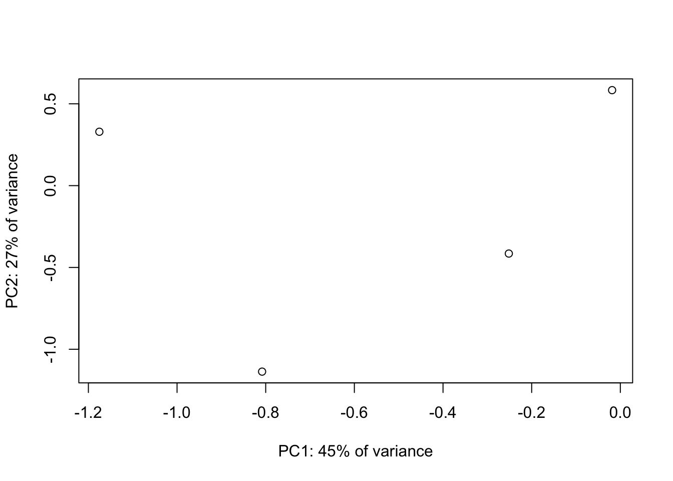
- BiPlots - projecting the original variable directions onto the new PC space. See
x <- pca
scores <- x$x
choices = 1L:2L
scale = 1
n <- NROW(scores)

lam <- x$sdev[choices]
lam <- lam * sqrt(n)
lam <- lam ^ scale
scores[, choices] / lam
## PC1 PC2
## Pt_a 0.18971007 0.05905298
## Pt_b 0.34894505 0.12743733
## Pt_c -0.40587967 -0.36622297
## Pt_d -0.12642641 -0.10445644
## Pt_e 0.19834344 -0.01851409
## Pt_f 0.33076958 -0.10502826
## Pt_g 0.43570084 0.15231731
## Pt_h -0.46315854 0.34516504
## Pt_i -0.04129107 -0.38315293
## Pt_j -0.58263254 0.46470891t(t(scores[, choices]) / lam)## PC1 PC2
## Pt_a 0.18971007 0.07723055
## Pt_b 0.26681466 0.12743733
## Pt_c -0.40587967 -0.47895305
## Pt_d -0.09666972 -0.10445644
## Pt_e 0.19834344 -0.02421306
## Pt_f 0.25291711 -0.10502826
## Pt_g 0.43570084 0.19920334
## Pt_h -0.35414599 0.34516504
## Pt_i -0.04129107 -0.50109435
## Pt_j -0.44549967 0.46470891# samples in PC space
#divided by lambda
t(t(x$rotation[, choices]) * lam)## PC1 PC2
## Var_1 0.5090406 -3.045506469
## Var_2 2.2782389 0.004638666
## Var_3 2.5817018 1.051389761
## Var_4 -2.4558879 0.478302155#original variable directions in PC space
#multiplied by lambdaAdditional resources on PCA
Tutorials
- Conceptual introduction to PCA by Laura Hamilton
- Why do we normalize the data before PCA
- PCA in python
- How to tell whether two groups are separate in PCA space with permutation of Euclidean distance between centroids - see supplementary data 2, section 2. (“Spatial clustering”) from Gertzung et al., 2017